The NWChem density functional theory (DFT) module uses the Gaussian basis set approach to compute closed shell and open shell densities and Kohn-Sham orbitals in the:
The formal scaling of the DFT computation can be reduced by choosing to use auxiliary Gaussian basis sets to fit the charge density (CD) and/or fit the exchange-correlation (XC) potential.
DFT input is provided using the compound DFT directive
  DFT
    ...
  END
The actual DFT calculation will be performed when the input module
encounters the TASK directive (Section 5.10).
TASK DFT
Once a user has specified a geometry and a Kohn-Sham orbital basis set the DFT module can be invoked with no input directives (defaults invoked throughout). There are sub-directives which allow for customized application; those currently provided as options for the DFT module are:
  VECTORS [[input] (<string input_movecs default atomic>) || \
                   (project <string basisname> <string filename>)] \
           [swap [alpha||beta] <integer vec1 vec2> ...] \
           [output <string output_filename default input_movecs>] \
           [lock]


  XC [[acm] [b3lyp] [beckehandh] [pbe0]\
     [becke97]  [becke97-1] [becke98] [hcth] [h120] [h147]\
      [h402] [becke97gga1] \
      [HFexch <real prefactor default 1.0>] \
      [becke88 [nonlocal] <real prefactor default 1.0>] \
      [xperdew91 [nonlocal] <real prefactor default 1.0>] \
      [xpbe96 [nonlocal] <real prefactor default 1.0>] \
      [gill96 [nonlocal] <real prefactor default 1.0>] \
      [xhcth  <real prefactor default 1.0>] \
      [lyp <real prefactor default 1.0>] \
      [perdew81 <real prefactor default 1.0>] \
      [perdew86 [nonlocal] <real prefactor default 1.0>] \
      [perdew91 [nonlocal] <real prefactor default 1.0>] \
      [cpbe96 [nonlocal] <real prefactor default 1.0>] \
      [chcth  <real prefactor default 1.0>] \
      [pw91lda <real prefactor default 1.0>] \
      [slater <real prefactor default 1.0>] \
      [vwn_1 <real prefactor default 1.0>] \
      [vwn_2 <real prefactor default 1.0>] \
      [vwn_3 <real prefactor default 1.0>] \
      [vwn_4 <real prefactor default 1.0>] \
      [vwn_5 <real prefactor default 1.0>] \
      [vwn_1_rpa <real prefactor default 1.0>]]


  CONVERGENCE [[energy <real energy default 1e-7>] \
               [density <real density default 1e-5>] \
               [gradient <real gradient default 5e-4>] \
               [dampon <real dampon default 0.0>] \
               [dampoff <real dampoff default 0.0>] \
               [diison <real diison default 0.0>] \
               [diisoff <real diisoff default 0.0>] \
               [levlon <real levlon default 0.0>] \
               [levloff <real levloff default 0.0>] \
               [ncydp <integer ncydp default 2>] \
               [ncyds <integer ncyds default 30>] \
               [ncysh <integer ncysh default 30>] \
               [damp <integer ndamp default 70>] [nodamping] \
               [diis [nfock <integer nfock default 10>]] \
               [nodiis] [lshift <real lshift default 0.5>] \
               [nolevelshifting] \
               [hl_tol <real hl_tol default 0.1>]]


  GRID [(xcoarse||coarse||medium||fine||xfine) default medium] \
       [(gausleg||lebedev ) default lebedev ] \
       [(old||new) default new ] \
       [(becke||erf1||erf2||ssf) default erf1] \
       [(euler||mura||treutler||lindh) default mura] \
       [rm <real rm default 2.0>]


  TOLERANCES [[tight] [tol_rho <real tol_rho default 1e-10>] \
              [accCoul <integer accCoul default 10>] \
              [radius <real radius default 25.0>]]


  DECOMP
  DFT||ODFT
  DIRECT
  INCORE
  ITERATIONS <integer iterations default 30>
  MAX_OVL
  MULLIKEN
  MULT <integer mult default 1>
  NOIO
  PRINT||NOPRINT
The following
sections describe these keywords and
optional sub-directives that can be specified for a DFT calculation
in NWChem.
The DFT module requires at a minimum the basis set for the Kohn-Sham
molecular orbitals. This basis set must be in the default basis set named
"ao basis", or it must be assigned to this default name using the
SET directive (see Section 5.7).
In addition to the basis set for the Kohn-Sham orbitals,
the charge density fitting basis set can also be specified in the
input directives for the DFT module. This basis set is used for the
evaluation of the Coulomb potential in the Dunlap scheme11.1.
The charge density fitting basis set must have the name "cd basis".
This can be the actual name of a basis set, or a basis set can be
assigned this name using the SET directive, as described in
Section 5.7. If this basis set is not defined by input,
the ![]() y exact Coulomb contribution is computed.
y exact Coulomb contribution is computed.
The user also has the option of specifying a third basis set for the evaluation of the exchange-correlation potential. This basis set must have the name "xc basis". If this basis set is not specified by input, the exchange contribution (XC) is evaluated by numerical quadrature. In most applications, this approach is efficient enough, so the "xc basis" basis set is not generally required.
For the DFT module, the input options for defining the basis sets in a given calculation can be summarized as follows;
The VECTORS directive is the same as that in the SCF module
(Section 10.5). Currently, the LOCK keyword
is not supported by the DFT module, however the directive
MAX_OVLhas the same effect.
  XC [[acm] [b3lyp] [beckehandh] [pbe0]\
     [becke97]  [becke97-1] [becke98] [hcth] [h120] [h147] \
      [h402] [becke97gga1] \
      [HFexch <real prefactor default 1.0>] \
      [becke88 [nonlocal] <real prefactor default 1.0>] \
      [xperdew91 [nonlocal] <real prefactor default 1.0>] \
      [xpbe96 [nonlocal] <real prefactor default 1.0>] \
      [gill96 [nonlocal] <real prefactor default 1.0>] \
      [xhcth  <real prefactor default 1.0>] \
      [lyp <real prefactor default 1.0>] \
      [perdew81 <real prefactor default 1.0>] \
      [perdew86 [nonlocal] <real prefactor default 1.0>] \
      [perdew91 [nonlocal] <real prefactor default 1.0>] \
      [cpbe96 [nonlocal] <real prefactor default 1.0>] \
      [chcth  <real prefactor default 1.0>] \
      [pw91lda <real prefactor default 1.0>] \
      [slater <real prefactor default 1.0>] \
      [vwn_1 <real prefactor default 1.0>] \
      [vwn_2 <real prefactor default 1.0>] \
      [vwn_3 <real prefactor default 1.0>] \
      [vwn_4 <real prefactor default 1.0>] \
      [vwn_5 <real prefactor default 1.0>] \
      [vwn_1_rpa <real prefactor default 1.0>]]
The user has the option of specifying the exchange-correlation
treatment in the DFT Module. The default exchange-correlation
functional is defined as the local density approximation (LDA) for
closed shell systems and its counterpart the local spin-density (LSD)
approximation for open shell systems. Within this approximation the
exchange functional is the Slater ![]() functional (from
J.C. Slater, Quantum Theory of Molecules and Solids, Vol. 4: The
Self-Consistent Field for Molecules and Solids (McGraw-Hill, New
York, 1974)), and the correlation functional is the Vosko-Wilk-Nusair
(VWN) functional (functional V) (S.J. Vosko, L. Wilk and M. Nusair,
Can. J. Phys. 58, 1200 (1980)). The parameters used in this
formula are obtained by fitting to the Ceperley and
Alder11.2Quantum Monte-Carlo solution of the homogeneous electron gas.
functional (from
J.C. Slater, Quantum Theory of Molecules and Solids, Vol. 4: The
Self-Consistent Field for Molecules and Solids (McGraw-Hill, New
York, 1974)), and the correlation functional is the Vosko-Wilk-Nusair
(VWN) functional (functional V) (S.J. Vosko, L. Wilk and M. Nusair,
Can. J. Phys. 58, 1200 (1980)). The parameters used in this
formula are obtained by fitting to the Ceperley and
Alder11.2Quantum Monte-Carlo solution of the homogeneous electron gas.
These defaults can be invoked explicitly by specifying the following keywords within the DFT module input directive,
XC slater vwn_5
The DECOMP directive causes the components of the energy
corresponding to each functional to be printed, rather than just the
total exchange-correlation energy which is the default.
Many alternative exchange and correlation functionals are available to the user. The following sections describe these options.
There are six exchange functionals in addition to the default exchange functional. These are
XC becke88
XC xperdew91
XC xpbe96
XC gill96
XC xhcth
XC HFexch
Note that the user also has the ability to include only the local or
nonlocal contributions of a given functional. In addition the user
can specify a multiplicative prefactor (the variable
<prefactor> in the input) for the local/nonlocal component or
total. An example of this might be,
XC becke88 nonlocal 0.72The user should be aware that the Becke88 local component is simply the Slater exchange and should be input as such.
Any combination of the supported exchange functional options can be used. For example the popular Gaussian B3 exchange could be specified as:
XC slater 0.8 becke88 nonlocal 0.72 HFexch 0.2
In addition to the default vwn_5 correlation functional, the user has
10 alternative correlation functionals to choose from: lyp, perdew81,
perdew86, perdew91, pw91lda, vwn_1, vwn_2, vwn_3,
vwn_4, and vwn_1_rpa.
As in the exchange functional input, individual local/nonlocal components as well as multiplicative prefactors can be invoked where appropriate. Each of the correlation functionals is listed below along with appropriate citation.
   XC vwn_1
   XC vwn_2
   XC vwn_3
   XC vwn_4
   XC vwn_5
Note that functionals; vwn_2, vwn_3, and vwn_4
require both sets of parameters (the Monte Carlo parameters of
Ceperley and Alder and VWN's RPA parameters) used in fitting the
homogeneous electron gas correlation energy. Functionals
vwn_1 and vwn_5 require only the Monte Carlo fitting
parameters. In order to reproduce results in the literature another
functional was added; the vwn_1_rpa. This is the original
vwn_1 functional with RPA parameters as opposed to the
prescribed Monte Carlo parameters. This functional can be invoked
with the keyword,
XC vwn_1_rpa
XC perdew81
XC pw91lda
XC perdew86
pw91lda local
correlation functional. This functional can be invoked with the keyword,
XC perdew91
XC cpbe96
XC chcth
XC lyp
Any combination of the supported correlation functional options can be used. For example B3LYP could be specified as:
XC vwn_1_rpa 0.19 lyp 0.81 HFexch 0.20 slater 0.80 becke88 nonlocal 0.72
In addition to the options listed above for the exchange and correlation functionals, the user has the alternative of specifying combined exchange and correlation functionals. The available hybrid functionals consist of the Becke ``half and half'' (see A.D. Becke, J. Chem. Phys. 98, 1372 (1992)), the adiabatic connection method (see A.D. Becke, J. Chem. Phys. 98, 5648 (1993)), b3lyp (popularized by Gaussian9X), Becke 1997 (``Becke V'' paper: A.D.Becke, J. Chem. Phys., 107, 8554 (1997)
These options can be invoked by specifying any of the following input lines,
   XC beckehandh
   XC acm
   XC b3lyp
   XC becke97
   Xc becke97-1
   xc becke98
   xc pbe0
   xc hcth
   xc h120
   xc h147
   xc h402
   xc becke97gga1
The keyword beckehandh specifies that the exchange-correlation energy will be
computed as
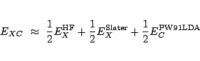
The keyword acm specifies that the exchange-correlation energy
is computed as
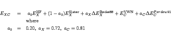
The keyword b3lyp specifies that the exchange-correlation energy
is computed as
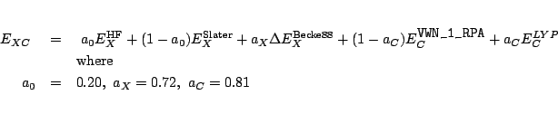
The keyword becke97-1 specifies the hybrid exchange-correlation energy
derived by Handy et al by re-fitting the Becke 1997 functional
(F.A.Hamprecht, A.J.Cohen, D.J.Tozer and N.C.Handy,
J. Chem. Phys. 109, 6264 (1998))
The keyword hcth specifies the exchange-correlation energy
functional derived by Hamprecht-Cohen-Tozer-Handy
(this is not a hybrid functional)
(F.A.Hamprecht, A.J.Cohen, D.J.Tozer and N.C.Handy,
J. Chem. Phys. 109, 6264 (1998))
|
|
ITERATIONS <integer iterations default 30>
The default optimization in the DFT module is to iterate on the
Kohn-Sham (SCF) equations for a specified number of iterations
(default 30). The keyword that controls this optimization
is ITERATIONS, and has the following general form,
iterations <integer iterations default 30>
The optimization procedure will stop when the specified number of iterations is reached or convergence is met.
  CONVERGENCE [energy <real energy default 1e-6>] \
              [density <real density default 1e-5>] \
              [gradient <real gradient default 5e-4>] \
              [hl_tol <real hl_tol default 0.1>]
              [dampon <real dampon default 0.0>] \
              [dampoff <real dampoff default 0.0>] \
              [ncydp <integer ncydp default 2>] \
              [ncyds <integer ncyds default 30>] \
              [ncysh <integer ncysh default 30>] \
              [damp <integer ndamp default 70>] [nodamping] \
              [diison <real diison default 0.0>] \
              [diisoff <real diisoff default 0.0>] \
              [(diis [nfock <integer nfock default 10>]) || nodiis] \
              [levlon <real levlon default 0.0>] \
              [levloff <real levloff default 0.0>] \
              [(lshift <real lshift default 0.5>) || nolevelshifting] \
Convergence is satisfied by meeting any or all of three criteria;
CONVERGENCE energy <real energy default 1e-6>
CONVERGENCE density <real density default 1e-5>
CONVERGENCE gradient <real gradient default 5e-4>
The default optimization strategy is to immediately begin direct inversion of the iterative subspace11.3. Damping is also initiated (using 70% of the previous density) for the first 2 iteration. In addition, if the HOMO - LUMO gap is small and the Fock matrix somewhat diagonally dominant, then level-shifting is automatically initiated. There are a variety of ways to customize this procedure to whatever is desired.
An alternative optimization strategy is to specify, by using the change in total energy (from iterations when N and N-1), when to turn damping, level-shifting, and/or DIIS on/off. Start and stop keywords for each of these is available as,
  CONVERGENCE  [dampon <real dampon default 0.0>] \
               [dampoff <real dampoff default 0.0>] \
               [diison <real diison default 0.0>] \
               [diisoff <real diisoff default 0.0>] \
               [levlon <real levlon default 0.0>] \
               [levloff <real levloff default 0.0>]
So, for example, damping, DIIS, and/or level-shifting can be turned on/off as desired.
Another strategy can be to simply specify how many iterations (cycles) you wish each type of procedure to be used. The necessary keywords to control the number of damping cycles (ncydp), the number of DIIS cycles (ncyds), and the number of level-shifting cycles (ncysh) are input as,
  CONVERGENCE  [ncydp <integer ncydp default 2>] \
               [ncyds <integer ncyds default 30>] \
               [ncysh <integer ncysh default 0>]
The amount of damping, level-shifting, time at which level-shifting is automatically imposed, and Fock matrices used in the DIIS extrapolation can be modified by the following keywords
  CONVERGENCE  [damp <integer ndamp default 70>] \
               [diis [nfock <integer nfock default 10>]] \
               [lshift <real lshift default 0.5>] \
               [hl_tol <real hl_tol default 0.1>]]
Damping is defined to be the percentage of the previous iterations density mixed with the current iterations density. So, for example
CONVERGENCE damp 70would mix 30% of the current iteration density with 70% of the previous iteration density.
Level-Shifting11.4 is defined as the
amount of shift applied to the diagonal elements of the unoccupied
block of the Fock matrix. The shift is specified by the
keyword lshift. For example the directive,
CONVERGENCE lshift 0.5causes the diagonal elements of the Fock matrix corresponding to the virtual orbitals to be shifted by 0.5 au. By default, this level-shifting procedure is switched on whenever the HOMO-LUMO gap is small. Small is defined by default to be 0.05 au but can be modified by the directive
hl_tol. An example of
changing the HOMO-LUMO gap tolerance to 0.01 would be,
CONVERGENCE hl_tol 0.01
Direct inversion of the iterative subspace with extrapolation of up to 10 Fock matrices is a default optimization procedure. For large molecular systems the amount of available memory may preclude the ability to store this number of N**2 arrays in global memory. The user may then specify the number of Fock matrices to be used in the extrapolation (must be greater than three (3) to be effective). To set the number of Fock matrices stored and used in the extrapolation procedure to 3 would take the form,
CONVERGENCE diis 3
Finally, the user has the ability to simply turn off any optimization procedures deemed undesirable with the obvious keywords,
CONVERGENCE [nodamping] [nodiis] [nolevelshifting]
  GRID [(xcoarse||coarse||medium||fine||xfine) default medium] \
       [(gausleg||lebedev ) default lebedev ] \
       [(old||new) default new ] \
       [(becke||erf1||erf2||ssf) default erf1] \
       [(euler||mura||treutler) default mura] \
       [rm <real rm default 2.0>]
A numerical integration is necessary for the evaluation of the exchange-correlation contribution to the density functional. The default quadrature used for the numerical integration is an Euler-MacLaurin scheme for the radial components (with a modified Mura-Knowles transformation) and a Lebedev scheme for the angular components. Within this numerical integration procedure various levels of accuracy have been defined and are available to the user. The user can specify the level of accuracy with the keywords; xcoarse, coarse, medium, fine, and xfine. The default is medium.
GRID [xcoarse||coarse||medium||fine||xfine]
Our intent is to have a numerical integration scheme which would give us approximately the accuracy defined below regardless of molecular composition.
| Keyword | Total Energy Target Accuracy |
| xcoarse | |
| coarse | |
| medium | |
| fine | |
| xfine |
In order to determine the level of radial and angular quadrature needed to give us the target accuracy we computed total DFT energies at the LDA level of theory for many homonuclear atomic, diatomic and triatomic systems in rows 1-4 of the periodic table. In each case all bond lengths were set to twice the Bragg-Slater radius. The total DFT energy of the system was computed using the converged SCF density with atoms having radial shells ranging from 35-235 (at fixed 48/96 angular quadratures) and angular quadratures of 12/24-48/96 (at fixed 235 radial shells). The error of the numerical integration was determined by comparison to a ``best'' or most accurate calculation in which a grid of 235 radial points 48 theta and 96 phi angular points on each atom was used. This corresponds to approximately 1 million points per atom. The following tables were empirically determined to give the desired target accuracy for DFT total energies. These tables below show the number of radial and angular shells which the DFT module will use for for a given atom depending on the row it is in (in the periodic table) and the desired accuracy. Note, differing atom types in a given molecular system will most likely have differing associated numerical grids. The intent is to generate the desired energy accuracy (with utter disregard for speed).
| Keyword | Radial | Theta | phi |
| xcoarse | 30 | 12 | 24 |
| coarse | 50 | 15 | 30 |
| medium | 70 | 18 | 36 |
| fine | 100 | 24 | 48 |
| xfine | 140 | 34 | 68 |
| Keyword | Radial | Theta | phi |
| xcoarse | 45 | 12 | 24 |
| coarse | 75 | 18 | 36 |
| medium | 95 | 24 | 48 |
| fine | 125 | 30 | 60 |
| xfine | 175 | 44 | 88 |
| Keyword | Radial | Theta | phi |
| xcoarse | 75 | 14 | 28 |
| coarse | 95 | 22 | 44 |
| medium | 110 | 30 | 60 |
| fine | 160 | 34 | 68 |
| xfine | 210 | 38 | 76 |
| Keyword | Radial | Theta | phi |
| xcoarse | 105 | 16 | 32 |
| coarse | 130 | 20 | 40 |
| medium | 155 | 32 | 64 |
| fine | 205 | 44 | 88 |
| xfine | 235 | 48 | 96 |
In addition to the simple keyword specifying the desired accuracy as
described above, the user has the option of specifying a custom
quadrature of this type in which ALL atoms have the same grid
specification. This is accomplished by using the gausleg keyword.
GRID gausleg <integer nradpts default 50> <integer nagrid default 10>
In this type of grid, the number of phi points is twice the number of theta points. So, for example, a specification of,
GRID gausleg 80 20would be interpreted as 80 radial points, 20 theta points, and 40 phi points per center (or 64000 points per center before pruning).
A second quadrature is the Lebedev scheme for the angular components11.5. Within this numerical integration procedure various levels of accuracy have also been defined and are available to the user. The input for this type of grid takes the form,
GRID lebedev <integer radpts > <integer iangquad >In this context the variable iangquad specifies a certain number of angular points as indicated by the table below.11.6
|
The user can also specify grid parameters specific for a given atom type:
parameters that must be supplied are: atom tag, number of radial points, number
of angular points and accQrad (all three parameters must be given).
As an example, here is a grid input line for the water molecule
grid lebedev 80 11 H 70 8 12 O 90 11 15
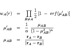
GRID [(becke||erf1||erf2||ssf) default erf1]
Erf![]() partionioning functions
partionioning functions
GRID [[euler||mura||treutler] default mura]
GRID [[old||new] default new]
In Nwchem 4.0 the XC integration code has been re-written using a space decomposiition scheme similar to the one proposed in R.E.Stratmann, G.Scuseria and M.J.Frisch, Chem. Phys. Lett. 257, 213 (1996) (keyword new).
To use the XC integration routines available in older version of NWChem, use the keyword old.
  TOLERANCES [[tight] [tol_rho <real tol_rho default 1e-10>] \
              [accCoul <integer accCoul default 10>] \
              [radius <real radius default 25.0>]]
The user has the option of controlling screening for the tolerances in
the integral evaluations for the DFT module. In most applications,
the default values will be adequate for the calculation, but different
values can be specified in the input for the DFT module using the
keywords described below.
The input
parameter accCoul is used to define the tolerance in Schwarz
screening for the Coulomb integrals. Only integrals with estimated
values greater than
![]() are evaluated.
are evaluated.
TOLERANCES accCoul <integer accCoul default 10>
Screening away needless computation of the XC functional (on the grid) due to negligible density is also possible with the use of,
TOLERANCES tol_rho <real tol_rho default 1e-10>XC functional computation is bypassed if the corresponding density elements are less than
tol_rho.
A screening parameter, radius, used in the screening of the
Becke or Delley spatial weights is also available as,
TOLERANCES radius <real radius default 25.0>where radius is the cutoff value in bohr.
The tolerances as discussed previously are insured at convergence.
More sleazy tolerances are invoked early in the iterative process
which can speed things up a bit. This can also be problematic at
times because it introduces a discontinuity in the convergence
process. To avoid use of initial sleazy tolerances the user can
invoke the tight option:
TOLERANCES tight
This option sets all tolerances to their default/user specified values at the very first iteration.
  DIRECT||INCORE
  NOIO
The inverted charge-density and exchange-correlation matrices
for a DFT calculation are normally written to disk storage. The user
can prevent this by specifying the keyword noio within the
input for the DFT directive. The input to exercise this option is
as follows,
noioIf this keyword is encountered, then the two matrices (inverted charge-density and exchange-correlation) are computed ``on-the-fly'' whenever needed.
The INCORE option is always assumed to be true but can be
overridden with the option DIRECT in which case all integrals
are computed ``on-the-fly''.
  DFT||ODFT
  MULT <integer mult default 1>
Both closed-shell and open-shell systems can be studied using
the DFT module. Specifying the keyword MULT within the DFT
directive allows the user to define the spin multiplicity of the system.
The form of the input line is as follows;
MULT <integer mult default 1>When the keyword
MULT is specified, the user can define the integer
variable mult, where mult is equal to the number of alpha
electrons minus beta electrons, plus 1.
The keywords DFT||ODFT were originally intended to specify
closed or open shell and are really unnecessary except in the context
of forcing a closed-shell system to be computed as an open shell
system (i.e., using a spin-unrestricted wavefunction).
sic [perturbative || oep || oep-loc <default perturbative>]
The Perdew and Zunger (see J. P. Perdew and A. Zunger, Phys. Rev. B 23, 5048 (1981)) method to remove the self-interaction contained in many exchange-correlation functionals has been implemented with the Optimized Effective Potential method (see R. T. Sharp and G. K. Horton, Phys. Rev. 90, 317 (1953), J. D. Talman and W. F. Shadwick, Phys. Rev. A 14, 36 (1976)). Three variants of these methods are included in NWChem:
print "SIC information"
MULLIKEN
Mulliken analysis of the charge distribution is invoked by the keyword:
MULLIKENWhen this keyword is encountered, Mulliken analysis of both the input density as well as the output density will occur.
PRINT||NOPRINT
The PRINT||NOPRINT options control the level of output in the
DFT. Known controllable print options are:
|